14 Walkthrough 8: Predicting student pass/fail outcomes using supervised machine learning
Abstract
This chapter introduces an increasingly common approach to modeling — supervised machine learning. This involves identifying an outcome or a dependent variable and training a model to predict an outcome. Some supervised machine learning models are highly complex, while others are simple. To illustrate this concept, this chapter includes a demonstration of using a generalized linear model to predict whether students will pass a class. The Open University Learning Analytics Dataset (OULAD) is used as example data in this activity. The {tidymodels} collection of packages is used to carry out the principal supervised machine learning steps. At the conclusion, ways to build more complex models are discussed.
14.2 Functions introduced
stats::quantile()rsample::initial_split()rsample::training()rsample::testing()recipes::recipe()parsnip::logistic_reg()parsnip::set_engine()parsnip::set_mode()workflows::workflow()tune::collect_predictions()tune::collect_metrics()
14.3 Vocabulary
We introduce these key terms in the chapter:
- supervised machine learning
- training data
- testing data
- overfitting
- generalizability
- bias-variance tradeoff
- logistic regression
- classification
- feature engineering
- recipe
- workflow
- stratified split
- predictions
- metrics
- confusion matrix
- sensitivity (recall) and specificity
- positive predictive value (PPV) and negative predictive value (NPV)
- AUC-ROC
14.4 Chapter overview
14.4.1 Background
In a face-to-face classroom, teachers use student cues to help them engage. In online classrooms, these cues aren’t always available.
For example, in a face-to-face class, teachers adjust when they notice that students are distracted. Many online educators look for ways to support students online in the same way that face-to-face instructors would. Technology provides new methods of collecting and storing data that can serve as the basis for this kind of student support.
Online Learning Management Systems (LMSs) automatically track student interactions with the system and feed that data back to the course instructor. The collection of this data is often met with mixed reactions from educators. Some are concerned that this kind of data collection is intrusive, but others see a new opportunity to support students in online classrooms. As long as data is collected and used responsibly, this kind of data collection can support student success.
In this walkthrough, you’ll examine the question, How well can we predict students who are at risk of dropping a course? To answer this question, you’ll use typical learning analytics data—student records, assessment outcomes, course outcomes, and measures of students’ interactions with the course.
Here’s the key shift in thinking you’ll make when using a supervised machine learning model: You’ll focus on predicting an outcome, like whether a student passes a course. This is different from explaining how variables influence an outcome, like how course time relates to final grades. You’ll learn to execute this shift in thinking through a generalized linear model.
14.4.2 Data sources
You’ll be using a widely-used dataset in the learning analytics field: the Open University Learning Analytics Dataset (OULAD). The OULAD was created by learning analytics researchers at the United Kingdom-based Open University (Kuzilek et al., 2017). It includes data from post-secondary learners’ participation in one of several Massive Open Online Courses. These courses are called modules in the OULAD.
Many students successfully complete these courses, but not all do. This highlights the importance of identifying those who may be at risk.
Our analysis will use three datasets, oulad_students, oulad_assessments, and oulad_interactions_filtered. The oulad_students dataset has undergone preprocessing to streamline the analysis. It uses information from three sources that relate to students and the courses they took: studentInfo, courses, and studentRegistration. The oulad_assessments file provides data on students’ performance on various assessments throughout their courses.
14.4.3 Methods
14.4.3.1 Predictive analytics and supervised machine learning
“Predictive analysis” is a buzzword in education software spheres. Administrators and educators alike are interested in applying the methods long utilized by marketers and other business professionals to predict what a person will want, need, or do. “Predictive analytics” is a blanket term that describes any statistical approach that yields a prediction. You could ask a predictive model: “What is the likelihood that my cat will sit on my keyboard today?” and, given enough past information about your cat’s computer-sitting behavior, the model estimates the probability of computer-sitting. Under the hood, some predictive models are not complex. In this chapter, you’ll use logistic regression, which is one of the simpler predictive models.
There is an adage: “garbage in, garbage out”. This holds true here. If you do not feel confident that the data you collected is accurate, you won’t feel confident in your conclusions, regardless of the model. To collect good data, you must first identify what you want to learn and what information you need to learn it.
Sometimes, people approach analysis from the opposite direction—they look at the data they have and identify questions that could be answered by it. That approach is okay, as long as you acknowledge that the pre-existing dataset may not contain all the information you need to answer your specific questions. You might need to find additional information to add to your dataset to truly answer the questions you have.
At its core, machine learning is the process of training a model to accurately predict on a training dataset (this is the “learning” part of machine learning). Then, this newly trained model is used on new data. At this point, you’ll evaluate how well the model worked outside of the training data conditions.
14.4.3.2 Prediction vs. explanation: same model, different goals
You may already be familiar with statistical models used to explain relationships between variables. For example, a researcher might use a regression model to estimate how strongly student motivation relates to course grades. The interesting output of that analysis is the coefficient itself: how much grades change with motivation, and whether that relationship is statistically significant.
Supervised machine learning can use the very same statistical model — including the logistic regression you’ll use in this walkthrough — but with a different aim. In a supervised machine learning approach, the interesting output isn’t the coefficients; it’s the predictions themselves. Rather than asking “how does motivation relate to grades?”, you’ll ask “how accurately can we predict each student’s grade?”
Let’s consider a regression equation (below) used to understand how a single variable (\(b_1\)) relates to an outcome (\(y\)). There is also an intercept term (\(b_0\)) and a residual term (\(e\)).
\[y = b_0 + b_1x_1 + \cdots + e\]
If your goal is inference, or explaining how variables relate to an outcome, you’ll typically use theory and prior research to choose a small set of predictors whose individual effects you can interpret. You’ll favor a transparent model where you understand how each predictor relates to \(y\).
If your goal is prediction, you can do things differently:
- You can include many more predictors than is typical in an explanatory model, since you care less about interpreting each one individually.
- Multicollinearity (predictors being correlated with one another) is less of a concern, since you’re not trying to make claims about the effect of any single predictor.
- You evaluate the model not by its R², or coefficient significance, but by how well a trained model predicts values in a separate test dataset.
- You can use much more complex models, accepting some loss of interpretability in exchange for better predictive accuracy.
The key idea is that it’s not about the algorithm, it’s about the aim and the use.
14.4.3.3 Why split data into training and testing sets?
A core practice of supervised machine learning is splitting your data into two parts: a training set used to fit the model, and a testing set used to evaluate how well the model predicts on data it hasn’t seen.
Why go through this trouble? If you fit a model using all of your data, you can almost always make the model fit that data extremely well — even perfectly. But a model that fits its own training data perfectly often performs poorly when given new data. This problem is called overfitting: the model has learned the specific patterns and noise of the training sample rather than patterns that generalize to new data.
There are real risks to skipping this step; indeed, if you see a machine learning model that does not do this, beware! If you never test your model on data it hasn’t seen, you can easily believe you have a much better model than you actually do. When you or someone using your model try to apply it to new students or new courses, the predictions can fall apart. That’s why training/testing splits aren’t optional for supervised machine learning — they’re how you evaluate whether what you’ve built is useful.
14.4.3.4 The bias-variance tradeoff
Whether your model generalizes well depends on a tradeoff that all models face called the bias-variance tradeoff:
- Bias is how far off your model’s predictions are from the true outcomes, on average. A model with high bias is under-fit — it fails to capture important relationships in the data.
- Variance is how much your predictions would change if you trained the model on a slightly different sample. A model with high variance is over-fit — it’s too tuned to the specific data it saw during training.
A simple model (like linear regression) tends to have higher bias but lower variance: it might miss subtle patterns, but its predictions are stable across different samples. A very complex model (like a deep neural network with many parameters) can fit training data very closely (low bias) but may give very different predictions when shown new data (high variance).
Good supervised machine learning practice balances the two — finding a model that captures real patterns in the data without latching onto noise. Splitting data into training and testing sets is one important way to check this balance.
14.4.3.5 A spectrum of interpretability
Models also vary in how easy they are to interpret. It can help to think of three rough categories:
- Transparent box models, like linear and logistic regression, have coefficients that map directly to interpretable effects. These are often preferred when inference is the goal.
- Gray box models, like decision trees and random forests, are more complex but still allow you to inspect things like which predictors matter most (“feature importance”). They sit in the middle.
- Black box models, like deep neural networks, can offer the highest predictive accuracy, but their internal logic is largely opaque.
In this chapter, you’ll start with a transparent model — logistic regression — because it makes the contrast between explanation and prediction especially clear. At the end of the chapter, you’ll see how to swap in more complex (gray box) models like random forests and boosted trees with only minor changes to your code.
Now you’ll dive into the analysis, starting with something you’re familiar with—loading packages.
14.5 Analysis
14.5.1 Load packages
If you have not installed any of these packages before, do so first using the install.packages() function. For a description of packages and their installation, review the Packages section of the Foundational Skills chapter.
14.6 The supervised machine learning workflow
Your goal in this walkthrough is to build a model that predicts whether a student is at risk of dropping out.
14.6.1 Step 1: Creating outcome and predictor variables
Feature engineering can be handled directly or through something called a “recipe.” How should you decide when to handle feature engineering directly or through a recipe? As you progress in your practice, you’ll be able to determine if it is more efficient to work outside of a recipe. You’ll also get more proficient at determining risks of working outside a recipe, like introducing “data leakage” that biases models. For now, this will not be an issue for the one you’ll be using in this walkthrough.
To begin, create the outcome variable (pass) and a factor variable for disability using mutate():
students <-
    students %>%
    mutate(pass = case_when(final_result == "Pass" ~ 1,
                            .default = 0)) %>%
    # Set "1" (pass) as the first level so {yardstick} treats it
    # as the positive class when computing sensitivity, specificity, etc.
    mutate(pass = factor(pass, levels = c("1", "0")),
           disability = as.factor(disability))
You will also summarize assessment data to create a new predictor for students’ performance on assessments submitted early in the course. Specifically, you’ll calculate the mean weighted score of assessments submitted before the first half of assignment dates.
code_module_dates <-
    assessments %>%
    group_by(code_module, code_presentation) %>%
    summarize(quantile_cutoff_date = quantile(date, probs = .5, na.rm = TRUE))
## `summarise()` has regrouped the output.
## ℹ Summaries were computed grouped by code_module and code_presentation.
## ℹ Output is grouped by code_module.
## ℹ Use `summarise(.groups = "drop_last")` to silence this message.
## ℹ Use `summarise(.by = c(code_module, code_presentation))` for per-operation
## grouping (`?dplyr::dplyr_by`) instead.assessments_joined <-
assessments %>%
left_join(code_module_dates) %>%
filter(date < quantile_cutoff_date) %>%
mutate(weighted_score = score * weight) %>%
group_by(id_student) %>%
summarize(mean_weighted_score = mean(weighted_score, na.rm = TRUE))## Joining with `by = join_by(code_module, code_presentation)`Last, you’ll create a socioeconomic status variable (imd_band), again outside the recipe:
students <-
    students %>%
    mutate(imd_band = factor(imd_band, levels = c("0-10%",
                                                  "10-20%",
                                                  "20-30%",
                                                  "30-40%",
                                                  "40-50%",
                                                  "50-60%",
                                                  "60-70%",
                                                  "70-80%",
                                                  "80-90%",
                                                  "90-100%"))) %>%
    mutate(imd_band = as.factor(imd_band))
Next, you’ll load a new file with interactions, or log-trace, data. This is the most granular data in the OULAD. In the OULAD documentation, this is called the virtual learning environment (VLE) data source. It’s a large file—even after taking a few steps to reduce its size. The file was prepared by only including interactions for the first one-third of the course.
Import the data using the {dataedu} package.
You’ll now explore the dataset to understand it better.
First, count() the activity_type variable and sort the resulting output by frequency.
##     activity_type       n
## 1         forumng 1279917
## 2         subpage 1104279
## 3       oucontent 1065736
## 4        homepage  832424
## 5        resource  436704
## 6            quiz  398966
## 7             url  232573
## 8          ouwiki   66413
## 9            page   33539
## 10  oucollaborate   25861
## 11   externalquiz   18171
## 12  questionnaire   16528
## 13   ouelluminate   13829
## 14       glossary    9630
## 15       dualpane    7306
## 16   htmlactivity    6562
## 17       dataplus     311
## 18  sharedsubpage     103
## 19 repeatactivity       6
You can see there is a range of activities students do. You may wish to explore this data in other ways, even beyond what you do for this exercise.
Think about how you would create a feature with sum_click. Think back to our discussion earlier; you have options for working with such time series data. Perhaps the simplest is to count the clicks.
Summarize the number of clicks for each student, specific to a single course. This means you’ll need to group your data by id_student, code_module, and code_presentation, before creating a
summary variable.
interactions_summarized <-
    interactions %>%
    group_by(id_student, code_module, code_presentation) %>%
    summarize(sum_clicks = sum(sum_click))
## `summarise()` has regrouped the output.
## ℹ Summaries were computed grouped by id_student, code_module, and
## code_presentation.
## ℹ Output is grouped by id_student and code_module.
## ℹ Use `summarise(.groups = "drop_last")` to silence this message.
## ℹ Use `summarise(.by = c(id_student, code_module, code_presentation))` for
## per-operation grouping (`?dplyr::dplyr_by`) instead.## # A tibble: 29,160 × 4
## # Groups: id_student, code_module [28,192]
## id_student code_module code_presentation sum_clicks
## <int> <chr> <chr> <int>
## 1 6516 AAA 2014J 999
## 2 8462 DDD 2013J 516
## 3 8462 DDD 2014J 10
## 4 11391 AAA 2013J 528
## 5 23629 BBB 2013B 84
## 6 23698 CCC 2014J 503
## 7 23798 BBB 2013J 277
## 8 24186 GGG 2014B 118
## 9 24213 DDD 2014B 642
## 10 24391 GGG 2013J 424
## # ℹ 29,150 more rowsHow many times did students click? Create a histogram to see. Use {ggplot2} and geom_histogram() to visualize the distribution of the sum_clicks variable you just created.
interactions_summarized %>%
    ggplot(aes(x = sum_clicks)) +
    geom_histogram(fill = dataedu_colors("darkblue"),
                   color = "black") +
  theme_dataedu()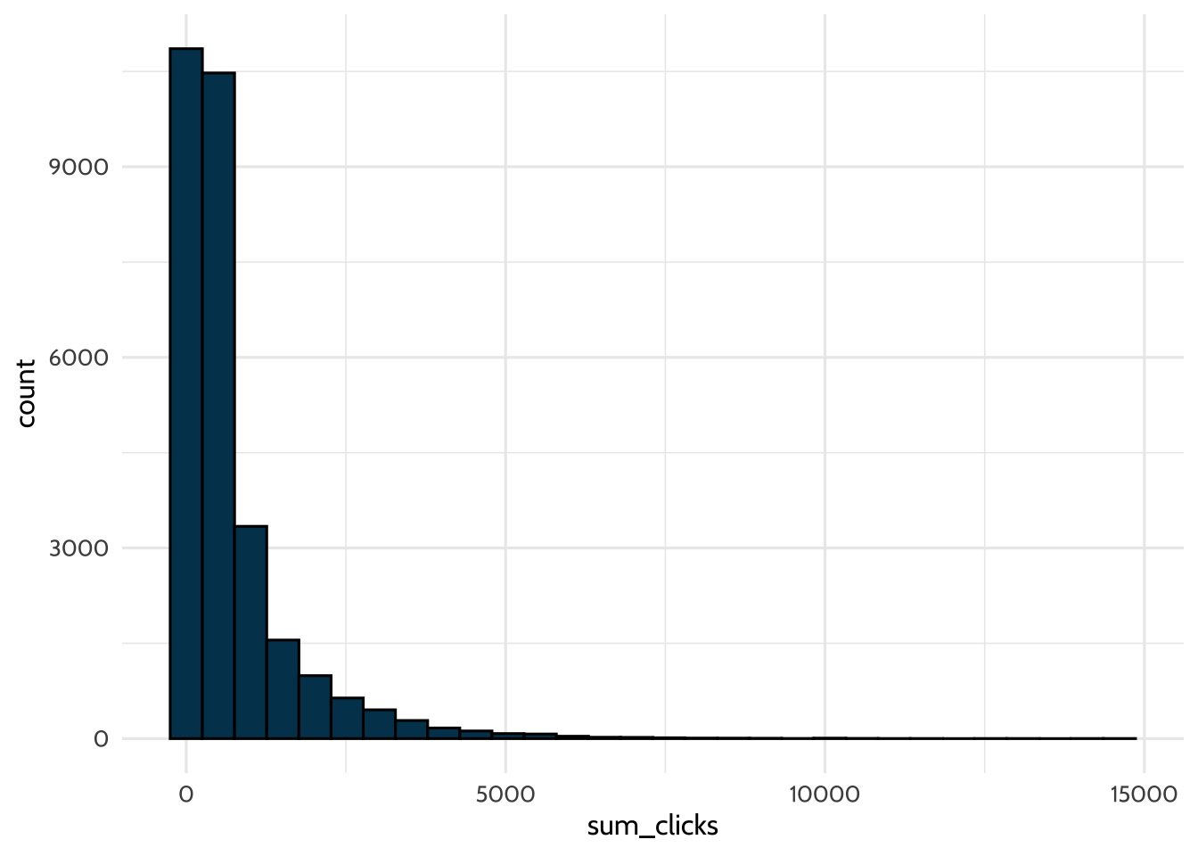
This is a good start — you’ve created the first feature based on the log-trace data, sum_clicks. What are some other features you can add? A benefit of using the summarize() function in R is that you can create multiple summary statistics at once.
Try calculating the standard deviation and mean of the number of clicks. Do this by copying the code you wrote above into the code chunk below and then add these two additional summary statistics.
interactions_summarized <-
    interactions %>%
    group_by(id_student, code_module, code_presentation) %>%
    summarize(sum_clicks = sum(sum_click),
              sd_clicks = sd(sum_click),
              mean_clicks = mean(sum_click))
## `summarise()` has regrouped the output.
## ℹ Summaries were computed grouped by id_student, code_module, and
## code_presentation.
## ℹ Output is grouped by id_student and code_module.
## ℹ Use `summarise(.groups = "drop_last")` to silence this message.
## ℹ Use `summarise(.by = c(id_student, code_module, code_presentation))` for
## per-operation grouping (`?dplyr::dplyr_by`) instead.Now join all of the data you’ll use for modeling: students, assessments_joined, and interactions_summarized.
Use left_join() twice, assigning the resulting output the name students_and_interactions.
14.6.2 Step 2: Splitting the data
As suggested above, a key step in supervised machine learning is splitting data into “training” and “testing” datasets. You’ll be using the training dataset to train the model. Then you’ll use the test dataset to evaluate the model’s performance. You’ll try the model you trained earlier, but this time on new test data. The outcome in this walkthrough is students passing the course in question.
You’ll split the dataset into training and testing sets using an 80-20 split. Generally, a split like this is appropriate with a larger dataset; for smaller datasets, something closer to a 50-50 split may be more appropriate. You’ll also conduct a stratified sample using the outcome variable — here, pass. Stratifying means that the training and testing sets will each contain roughly the same proportion of students who passed and didn’t pass as the full dataset does. Without stratification, a random split could end up with very different pass rates in training and testing, which would muddy your evaluation. Stratification is generally a good practice (Boehmke & Greenwell, 2019).
set.seed(2025) # As this step involves a random sample, setting the seed ensures the same result for pedagogical purposes

# Specify the proportion for the split
train_test_split <-
    initial_split(students_and_interactions, prop = 0.8, strata = "pass")

# Create the training data
data_train <-
    training(train_test_split)

# Create the testing data
data_test  <-
    testing(train_test_split)
14.6.3 Step 3: Creating a recipe for selected preprocessing steps
This is the recipe step mentioned earlier in the walkthrough. You’ll do two things here.
First, you’ll specify which predictor variables predict the outcome. For those familiar with the lm() function in R, this behaves similarly; the outcome goes on the left side of the ~, and predictors go on the right. Note that you’ll be using the training data for this.
Second, you’ll use step_() functions, which are for preprocessing. These are described in the comments below.
my_rec <-
    recipe(pass ~ disability + imd_band + mean_weighted_score +
                  num_of_prev_attempts + gender + region + highest_education +
                  sum_clicks + sd_clicks + mean_clicks,
           data = data_train) %>%
    # This step is to impute missing values for numeric variables
    step_impute_mean(mean_weighted_score, sum_clicks, sd_clicks, mean_clicks) %>%
    # This step is to impute missing values for categorical/factor variables
    step_impute_mode(imd_band) %>%
    # Center and scale these variables
    step_center(mean_weighted_score, num_of_prev_attempts) %>%
    step_scale(mean_weighted_score, num_of_prev_attempts) %>%
    # Dummy code all categorical/factor predictors
    step_dummy(all_nominal_predictors(), -all_outcomes())
Inspect the recipe to verify the steps you have specified:
## ## ── Recipe ──────────────────────────────────────────────────────────────────────## ## ── Inputs## Number of variables by role## outcome: 1
## predictor: 10## ## ── Operations## • Mean imputation for: mean_weighted_score, sum_clicks, sd_clicks, ...## • Mode imputation for: imd_band## • Centering for: mean_weighted_score num_of_prev_attempts## • Scaling for: mean_weighted_score num_of_prev_attempts## • Dummy variables from: all_nominal_predictors() -all_outcomes()14.6.4 Step 4: Specifying the model and workflow
Next, specify a logistic regression model and bundle the recipe and model into a workflow.
This step has a lot of pieces, but they are fairly boilerplate. First, specify the model:
my_mod <-
    logistic_reg() %>% # Specifies the type of model
    set_engine("glm") %>% # Specifies the package we use to estimate the model
    set_mode("classification") # Specifies whether we are classifying a dichotomous, categorical, or factor variable
Next, specify the workflow, which will stitch the recipe and model together:
You’re almost there!
14.6.5 Step 5: Fitting the model
Now you’ll fit the model to the training data. First, you’ll need to specify which metrics you want to calculate. These are statistics that will help you understand how good the model is at making predictions. You’ll use accuracy, plus four other metrics — sensitivity, specificity, positive predictive value (PPV), and negative predictive value (NPV) — that you’ll interpret in detail in Step 6.
Finally, you’ll fit the model. Do this by calling the last_fit() function on the workflow and the split specification of the data. You’ll also specify which metrics to use.
Note that while there are other fitting functions available, you’re using last_fit() to do two steps at once: fitting the model to the training data, then using the trained model to make predictions on the test data and compute the metrics you specified. This is why you pass train_test_split (the split object) rather than the data itself — last_fit() uses the split to know which rows are training and which are testing.
If you wanted to do these steps separately — for example, to inspect the fitted model before evaluating it — you could use fit() on the training data and then call predict() on the test data manually. For the purposes of this walkthrough, last_fit() is the cleaner option.
Other times, you may use cross-validation, where you’ll split the training data many times and fit the model to each of these splits. You’ll return to cross-validation briefly in the Conclusion. For more on the technique, consider reading Chapter 2 in (Boehmke & Greenwell, 2019).
14.6.6 Step 6: Evaluating model performance
You’ve fit the model — now the question is: how good are its predictions? The {tidymodels} package makes it straightforward to retrieve the metrics you specified earlier:
## # A tibble: 5 × 4
##   .metric  .estimator .estimate .config
##   <chr>    <chr>          <dbl> <chr>
## 1 accuracy binary         0.640 pre0_mod0_post0
## 2 sens     binary         0.172 pre0_mod0_post0
## 3 spec     binary         0.926 pre0_mod0_post0
## 4 ppv      binary         0.587 pre0_mod0_post0
## 5 npv      binary         0.647 pre0_mod0_post0
14.7 Interpreting results
How did the model do? Focus on accuracy for now: the model correctly predicted whether students passed around 64% of the time.
14.7.1 The limitation of accuracy
Accuracy is easy to interpret, but it can also be deceiving. Imagine that only 20% of students in a course actually pass. A model that always predicts “did not pass” — regardless of any input — would have 80% accuracy on this data, just because most students did not pass. That model would be useless for the actual purpose of identifying students who passed (or struggled), but its accuracy alone wouldn’t tell you that.
This is a general issue. Accuracy can be insufficient when:
- Outcomes are imbalanced (one class is much more common than the other).
- Different kinds of errors have different consequences.
- You need to tune your model for a specific purpose.
To get past these limitations, you need to look at which predictions the model got right and wrong.
14.7.2 Looking deeper with a confusion matrix
A confusion matrix is a 2 × 2 table that compares the model’s predictions against the true outcomes. It breaks the model’s predictions into four categories:
- True positive (TP): the student passed, and the model predicted “pass.”
- True negative (TN): the student did not pass, and the model predicted “did not pass.”
- False positive (FP): the student did not pass, but the model predicted “pass.”
- False negative (FN): the student passed, but the model predicted “did not pass.”
You can produce a confusion matrix directly from final_fit by collecting the test-set predictions and passing them to conf_mat():
##           Truth
## Prediction    1    0
##          1  426  300
##          0 2047 3747
The accuracy you saw earlier is just (TP + TN) divided by the total. But the confusion matrix lets you ask much sharper questions — and several useful metrics can be derived from its four cells.
14.7.3 Metrics built from the confusion matrix
The metrics below all come from rearranging the same four numbers in the confusion matrix, but each answers a different question.
| Metric | Equation | Question it answers |
|---|---|---|
| Accuracy | (TP + TN) / Total | What proportion of all predictions were correct? |
| Sensitivity (also called recall) | TP / (TP + FN) | Of all the students who actually passed, how many did the model correctly identify? |
| Specificity | TN / (TN + FP) | Of all the students who actually did not pass, how many did the model correctly identify? |
| Precision (also called positive predictive value, PPV) | TP / (TP + FP) | Of all the students the model predicted would pass, how many actually did? |
| Negative predictive value (NPV) | TN / (TN + FN) | Of all the students the model predicted would not pass, how many actually did not? |
Each of these appears in your collect_metrics() output, because you included them in my_metrics earlier. Look back at those values now in light of the table. The sensitivity value of around 0.17 tells you the model correctly identifies only a small share of students who actually passed — it misses most of them. The specificity value of around 0.93, by contrast, tells you the model correctly identifies most students who did not pass. The PPV of around 0.59 says that when the model does predict a student will pass, it’s right about 59% of the time; the NPV of around 0.65 says that when it predicts a student will not pass, it’s right about 65% of the time.
Together, these suggest the model is biased toward predicting “not pass” — it does well at flagging students who won’t pass, but misses many of the students who actually do pass. This pattern is common when the outcome is imbalanced: in our test set, more students did not pass than did, so a model that leans toward predicting “not pass” can achieve reasonable accuracy without being especially good at the harder task of identifying who will pass.
14.7.4 When does each metric matter?
Which of these metrics matters most depends entirely on the question you’re asking and the consequences of being wrong. Two examples make the point:
- If you’re using a model to flag students who might benefit from extra support, a false positive (flagging a student who didn’t actually need it) is relatively low-cost. You’d rather catch every student who needs help (high sensitivity) even at the cost of some false flags (lower PPV).
- If you’re using a model to make a high-stakes decision — say, automatically flagging students for academic dishonesty — false positives can do real harm to students who didn’t actually cheat. You’d want PPV to be very high before acting on a prediction, even if it means missing some real cases (lower sensitivity).
Your judgment as a researcher, and as someone who understands the context, is critical here. There is no metric that is uniformly “best.” The right metric is the one that aligns with how the model will be used and what kinds of errors are acceptable in that use.
14.7.5 Beyond the confusion matrix: AUC-ROC
You’ll also encounter another metric called AUC-ROC (Area Under the Curve - Receiver Operating Characteristic) in the supervised machine learning literature. The intuition is that a classification model usually produces a probability of belonging to a class (e.g., probability of passing), which is then converted to a yes/no prediction by applying a threshold (typically 0.5). AUC-ROC summarizes how well the model’s probabilities separate the two classes across every possible threshold, not just the default one. Values closer to 1.0 are better; 0.5 indicates a model that’s no better than chance. You don’t compute AUC-ROC here, but you can add roc_auc to your metric set if you want it.
14.7.6 Improving the model
On the question of how to improve the model: one benefit of the {tidymodels} framework is swapping in different algorithms with very few changes to your code. Try one of these modifications for a random forest and a boosted tree model and see how the predictive performance changes. How much better do these models do? Are the gains in accuracy overall, or in particular metrics like sensitivity or PPV?
14.8 Conclusion
Though this is a relatively simple model, many of the ideas explored in this chapter will prove useful for other machine learning methods. The goal is for you to finish this walkthrough with the confidence to explore using machine learning to answer a question or to solve a problem of your own in the areas of teaching, learning, and educational systems.
Here are several natural directions to go from here:
More careful feature engineering. In this walkthrough, you summarized the log-trace (interactions) data with three simple statistics: the sum, standard deviation, and mean of clicks per student. There’s a lot more you can do with this kind of time-series data. You could compute clicks within specific time windows (e.g., the first week of the course vs. the week before an assessment), count distinct activity types a student engaged with, or capture how a student’s activity pattern changes over time. Each of these is a different feature you can engineer, and good feature engineering is often what separates a so-so SML model from a strong one.
Cross-validation. The chapter used a single train/test split. A more robust approach is cross-validation: split your training data into several “folds” (typically 5 or 10), fit the model many times with each fold held out as a temporary validation set, and average the resulting metrics. This gives a more stable estimate of how well your model is likely to perform on new data, and is especially useful when you’re trying different models or tuning their parameters. The {tidymodels} packages support this with vfold_cv() and fit_resamples().
More complex models. At the end of Step 6, you saw how to swap in a random forest or a boosted tree model with only a few lines of code. These gray box models (per the spectrum of interpretability discussed in the Methods section) can often capture patterns that logistic regression cannot — but they also have parameters that need to be tuned to perform well. Tuning is usually done in combination with cross-validation, using functions like tune_grid() from the {tune} package.
In this chapter, we introduced general machine learning ideas in the context of predicting students’ passing a course. Like many of the topics in this book, there is much more to discover. We encourage you to consult the books and resources in the Learning More chapter for more about machine learning methods.